Solvers
![]()
A range of calculation methods (solvers) are offered. Each given solver is applicable to certain classes of problems, and the correct method should be chosen for a given problem. A full description of the solvers is beyond the scope of this document, and the interested reader is referred to the references.
Split low/high frequency solvers
Different solvers may be chosen for the low and high frequency ranges. The crossover frequency is chosen via the Frequencies and Solvers page. A typical usage would be dBSeaModes for the low frequency range and dBSeaRay for the high. The crossover frequency is given broadly as
where f is the frequency in Hz, d is the average depth in meters, and c is the speed of sound (meters/second). Some experimentation may be required where the depth varies greatly.
Added to the solver-calculated transmission loss is the attenuation with distance in seawater. This is insignificant at low frequencies and in the human audio range, but at high frequencies, it can be significant. For example, attenuation is approximately 30 dB/km at 100 kHz. The attenuation with frequency is graphed on the water page.
20 log
Transmission loss is calculated based on simple geometric spreading, i.e., an inverse square law. The calculated attenuation is spherically symmetric and frequency independent. Bathymetry is ignored.
10 log
Transmission loss is calculated according to the \(20 \log \frac{r}{r_0}\) inverse square law, until the distance from the source is greater than the water depth at the source. From this point, levels drop according to \(10 \log \frac{r}{r_d}\), i.e., an inverse law. It is considered that the reflections from the seafloor and the sea surface constrain the sound energy within the water layer, and the problem becomes essentially 2-dimensional, or similar to a vertical line source extending from the surface to the seafloor. Axially symmetric, frequency independent. Bathymetry is ignored, with the exception of the aforementioned calculation based on the water depth at the source.
dBSeaPE - parabolic equation method
The dBSeaPE solver utilizes the so-called parabolic equation and is range-dependent, i.e., it takes variable bathymetry into account. dBSeaPE is suitable for low-frequency problems. The input to the solver is configured so that the sediment layer is extended down to 2 times the depth of the water column, with the attenuation rapidly increasing at the lowest depths. The intention is to remove energy that would be reflected from the very bottom of the sediment layer. The sea surface is a pressure-release interface.
As sharp discontinuities in density cause incorrect calculation results, the density is smoothed between water and seabed, and between seabed layers by means of a hyperbolic tangent function.
dBSeaModes - normal modes method
The normal modes are calculated for each water depth, based on the sediment properties and water sound speed profile. The sound field is calculated based on coupling between the calculated modes across the interfaces between different depths. The calculation is of the adiabatic, single forward scattering type. The overlying space is modeled as a vacuum. dBSeaModes is suitable where the frequency is low and/or the water depth is shallow. The sediment layer is extended well below the depth of the water column, with the attenuation rapidly increasing at the lowest depths. In this way, there are no modes where energy is reflected from the very bottom of the sediment layer (the space underneath the bottom of the sediment is also a vacuum). The maximum number of modes to include in the solution may be limited via the page Preferences → Solver advanced. If the value is set to 0, the solver uses all the modes found by the eigenvalue search routine.
dBSeaRay - ray tracing method
The ray solver forms a solution by tracing rays from the source out into the sound field. A large number of rays leave the source covering a range of angles, and the sound level at each point in the receiving field is calculated by summing the components from each individual ray. The number of rays and the method of summing (coherent or incoherent) may be set on the page Preferences → Solver advanced. Setting this number to 0 instructs the solver to choose the number of rays itself, however, it is often the case that the number of rays chosen is too high, leading to excessive computation time. It is often useful to set this number very low as a fast initial 'checking' solve, before increasing the number of rays and running a full solve which may take some time. The overlying space is modeled as a vacuum. dBSeaRay is suitable for high-frequency problems.
When multiple seafloor layers are present, rays are not split and traced into the seafloor. A complex reflection coefficient is calculated which is representative of the underlying layers, and this coefficient is applied to the ray at the point of seafloor reflection. The calculation of the reflection coefficient follows Computational Ocean Acoustics. Jensen et al., Springer, 2011 (section 1.6).
dBSeaRay is used for time-domain calculations. Instead of returning a transmission loss at each point in the slice, a list of ray arrivals is returned (with separate entries for each frequency). These arrivals lists can be used to calculate the effective time series at each point in the slice, which is then used to calculate peak, peak-to-peak, and frequency band SEL levels.
These calculation methods are extensively documented in Computational Ocean Acoustics. Jensen et al., Springer, 2011.
Postprocessing of levels for each source
After a solve, the calculated transmission losses for each source are post-processed. These steps are optional, and can be controlled from the page Preferences → Solver advanced. The transmission loss is made to decrease monotonically with increased distance from the source (i.e., the level will decrease with distance from the source). In addition, the transmission loss is averaged radially about the source. Averaging is performed with a normalized triangular kernel of length 2m + 1, where m is the [Radial smoothing factor selected on the page Preferences → Solver], on the calculated transmission losses moving radially around the source, for each range distance from the source. This option is useful when dealing with results from a solver that change rapidly in the radial direction.
To disable these postprocessing steps, set [Radial smoothing factor] to 0 and uncheck [Levels must decrease with distance from source].
Neither of these options has any effect when using the 10 log or 20 log solvers.
Interpolating levels from sources to the grid
For each source, sound levels are calculated in 'slices' radiating out from the source. The number of slices to calculate and the number of range points along each slice can be changed on the page Setup. These sound levels are then interpolated onto the rectangular problem grid. Therefore, at large distances from a source, there may be a significant spacing between the calculated slices. If more detail is required in such an area, then the number of solution slices should be increased.
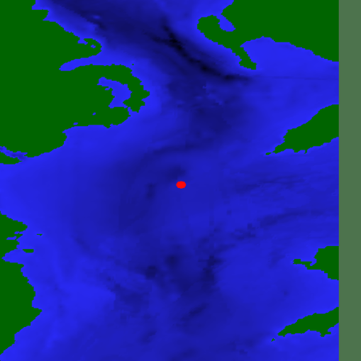
Image 1. A single source in the problem area.
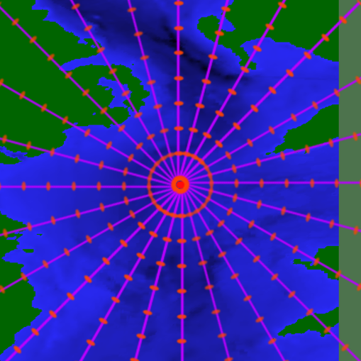
Image 2. The slices and solution points radiating out from the source.
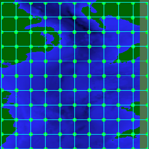
Image 3. Example problem grid.
The overall sound levels are interpolated (and summed over all active noise sources) to the rectangular problem grid.