Problem setup

Setting up the overall project world
A problem consists of the following elements:
- Bathymetry. Bathymetry is the gridded data representing the seafloor. At each point in the grid, a depth (or if negative, a land height) is given.
- Scenarios, containing:
- Sources. Sources represent the sound sources within the problem. A problem can have any number of sources, each producing a given sound spectrum or time series.
- Grid. The grid represents the entire problem area, in which sound levels are to be calculated. Points are evenly distributed in the x and y directions and sound levels are assessed at those points, by summing the contribution from each source.
- Probes. Probes are used to show the sound level and spectrum at particular points in the grid, and may be thought of as hydrophones. The grid may contain one or more probes.
- Water sound speed profile. The water sound speed profile represents the speed of sound in the water column.
- Sediment. Sediment gives the fluid properties of each of the layers in the seabed: density, speed of sound and attenuation. The seabed can have any number of layers.
- Weighting. Weightings represent the hearing of different marine species, against which the calculated sound levels are compared, giving a weighted sound level. The database contains both M weightings and species-specific hearing thresholds. More weightings may be added to the database if desired.
Problem creation
dBSea initially loads with some sample bathymetry data, showing an area of the Irish Sea and surrounding land. When creating a new problem, the bathymetry data is set to be all flat, at a depth of 100 meters. New bathymetry data may be imported from a CSV file. This can be done via View menu → Load bathymetry CSV.
CSV files can be created in most spreadsheet programs or may be created and edited using the included CSV Editor program. Each pixel is a depth in metres, separated by a semicolon. Example files may be found in the program directory. For more information on reading CSV data see the page Importing CSV data.
A very large amount of bathymetry data can slow down the program graphics. If this is the case, then the graphical bathymetry data may be reduced (Preferences → Graphics → Max bathymetry graphics data). This reduces the amount of graphics processing required, while the underlying calculation retains the bathymetry data at full accuracy. The bathymetry layer is cached by the graphics layer, so while the first draw of new bathymetry may be slow, subsequent draws are much faster and therefore the size of imported bathymetry is seldom a problem in practice.
Properties map
This map allows you to manage points for which you have information about the sound speed profile and the seabed properties. You can name and add comments to your selected locations (double click will place marker at mouse location on the map). If you have many points and properties, they can be imported from a JSON file. To set the actual values at the selected location see the page Water and the page Sediment.
Alternatively, use a JSON file to import many points in and automated fashion. Below is an example of an import:
[{
      "easting": 1234,
      "northing": 5.678e3,
      "name": "A name",
      "comments": "Some comments",
      "colour": "#ff0000",
      "water": {
            "temperature": 20,
            "salinity": 35,
            "velocity": 10,
            "direction": 1.2e-01,
            "name": "A name",
            "comments": "Some comments"
      },
      "ssp": {
            "cProfile": {
                  "depth": [0, 10, 15, 20, 55],
                  "c": [1500, 1510, 1520, 1510, 1500]
            },
            "name": "A name",
            "comments": "Some comments"
      },
      "seabed": {
            "name": "Seabed name",
            "comments": "Seabed comments",
            "isReferencedFromSeafloor": true,
            "layers": [
                  {
                        "depth": 0,
                        "name": "A name",
                        "comments": "Some comments",
                        "material": {
                              "c": 1700,
                              "density": 1500,
                              "attenuation": 0.1,
                              "name": "A name",
                              "comments": "Some comments"
                        }
                  },{
                        "depth": 10,
                        "name": "A name",
                        "comments": "Some comments",
                        "material": {
                              "c": 1820,
                              "density": 1810,
                              "attenuation": 0.05,
                              "name": "A name",
                              "comments": "Some comments"
                        }
                  }
            ]
      }
},
{
      "easting": 12342,
      "northing": 56782,
      "name": "A name2",
      "comments": "Some comments2",
      "colour": "#00ff00",
      "water": {
            "temperature": 5,
            "salinity": 3,
            "velocity": 2.7,
            "direction": 0.2,
            "name": "A name",
            "comments": "Some comments"
      },
      "ssp": {
            "cProfile": {
                  "depth": [0, 10],
                  "c": [1500, 1530]
            },
            "name": "A name",
            "comments": "Some comments"
      },
      "seabed": {
            "name": "Seabed name 2",
            "comments": "Seabed comments 2",
            "isReferencedFromSeafloor": true,
            "layers": [
                  {
                        "depth": 0,
                        "name": "A name",
                        "comments": "Some comments",
                        "material": {
                              "c": 2510,
                              "density": 2000,
                              "attenuation": 0.1,
                              "name": "A name",
                              "comments": "Some comments"
                        }
                  },{
                        "depth": 20,
                        "name": "A name",
                        "comments": "Some comments",
                        "material": {
                              "c": 2400,
                              "density": 2500,
                              "attenuation": 0.05,
                              "name": "A name",
                              "comments": "Some comments"
                        }
                  }
            ]
      }
}]
Notes on JSON files:
- Name, comments and colour fields are optional, other fields are not.
- Colour fields accept html-style colour codes.
- Numerical fields may be entered as
1234.567,1.234e3,987.6e-05and other variations on scientific notation. - The outermost list, between
[and], may be extended to include any number of entries. - Sound speed profiles (SSPs):
- The number of entries in
depthandcmust match, however different locations can have different lengths. - When interpolating SSPs, shorter lists have entries added as needed, via linear interpolation or nearest neighbour (when extrapolating). The scenario-wide depth list is the union of all depths entered.
- Interpolation of sound speed within SSPs is inverse distance weighting.
- Example:
- The number of entries in
"ssp": {
   "cProfile": {
     "depth": [0, 10, 20],
     "c": [1500, 1510, 1520]
   },
   "name": "SSP_one",
   "comments": "one SSP"
 }

 "ssp": {
   "cProfile": {
     "depth": [5, 15, 25],
     "c": [1505, 1510, 1520]
   },
   "name": "SSP_two",
   "comments": "another SSP"
 }
SSP at midpoint between SSP_one and SSP_two is:
{ "depth": [0, 5, 10, 15, 20, 25],
  "c": [1502.5, 1505, 1508.75, 1512.5, 1517.5, 1520]
}
Sea bed
- Density is in \(\mathrm{kg/m3}\)
- Each entry must have the same number of seabed layers, and the layers must appear in order of increasing depth.
- Layers of thickness
0are allowed and are achieved by setting the layer depth the same depth as the preceding layer. - Seabed properties, including depth of layer, are interpolated via inverse distance weighting.
Feel free to use the above example as a template to ensure correct syntax and field inclusion.
Shape Overlays
From dBSea 2.0 you can import shapefiles .shp & .shx into dBSea. As dBSea work from northing and easting, the location of your shapefiles will be most accurate if they are using this system too. If your shapefiles are in lat/lon format, dBSea will use the UTM-zone of the centre of the bathymetry to convert the lat/lon coordinates into northing and easting. This process may skew your shapefiles if the UTM zone does not match, or the bathymetry area is very large.
Setup cross section
Clicking the Setup cross-section button shows the current cross section location in the 3D view. The endpoints of the cross section may be dragged to the desired location. Once the location is selected, clicking the Show cross-section button ![]() in the main toolbar changes to cross-section view.
in the main toolbar changes to cross-section view.
If you have multiple sources in your scenario, the endpoint of the cross section can be made to jump to any source using the number 1-9 as index for the first 9 sources in your scenario.
The cross-section can also be specified by entering two points in the Set up cross section > Coordinates menu.
Set world scale
Setting the world scale tells the program the overall size of the problem area. Clicking the Set world scale button resets the 3D view. The user then clicks on two known points in the project area, and enters the distance between them, or the absolute locations of the two given points. This scales the overall size of the project area, and if absolute positions are given, also sets the project Northing and Easting. Instead of clicking on the first point, pressing the number keys (1, 2, 3...) will set the first point to the location of the corresponding source, if one exists.
Northing and Easting
The lowest left corner of the project area is initially situated at 0,0. Adding Northing and Easting changes the location of the project area. This function may be useful when matching locations given in different coordinate systems.
If the imported bathymetry was geotagged, dBSea will choose a suitable projection for the data, based on the UTM zone of the centre of the map. dBSea uses the expanded notation for UTM zones, meaning that all places have a numerical code (01-60) counting from the meridian at 180 degrees west to the meridian at 180 degrees east in 6 degree increments, and an alphabetical code based on latitude (C-X, omitting "I" and "O").
Note that some official UTM zones don't follow this grid, around Norway and Svalbard. dBSea ignores this and calculates zones as if the grid was not distorted in those areas. In addition zones A, B, Y and Z are not covered.
See this map (interactive) for UTM grid with coordinates (uses Google Maps/Earth). Alternatively download the ESRI shapefile.

Image 2. UTM Zones of the world
Grid setup
On the problem setup page, the number of grid points may be altered. The grid is rectilinear (Image 3), and the number of points may be altered in the x, y and z (depth) directions. The same z spacing is used for source solutions as for the grid.
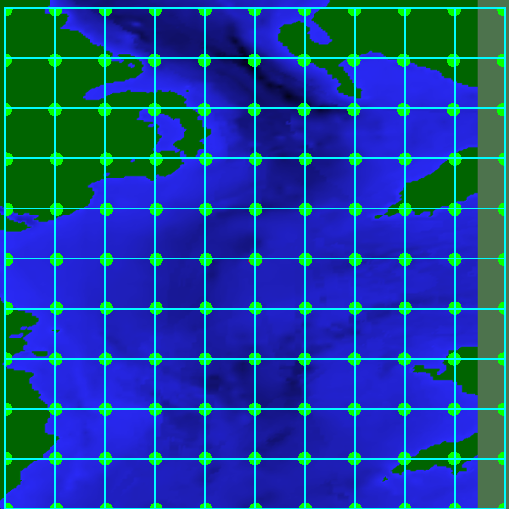
Image 3. Example problem grid in plan view.
dBSea does not require the x and y grid spacing to match, however this can be an issue when exporting levels. If the x and y spacing are sufficiently close, ESRI Ascii grid exported levels will use the standard CELLSIZE parameter and effectively give square cells. If the x and y spacing differ by too large a factor, the non-standard DX and DY parameters are used for the output file. These parameters are not supported by all GIS software, so check with your GIS package as to whether this data will work. A square aspect ratio can be ensured by clicking on Square aspect ratio.
Alternatively, use the button Set to map resolution, dBSea will match the calculation grid to the resolution of the bathymetry. Remember to check that you are happy with the resolution by inspecting Step sizes.
Source setup
The number of radial solution slices about each source and the evaluation range points along those slices (Image 4) may be altered on the problem setup page.
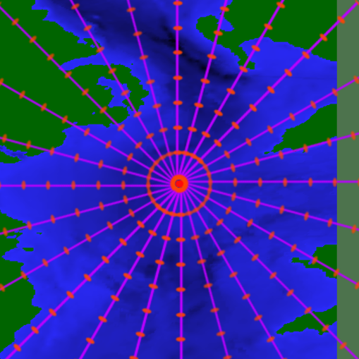
Image 4. Example source with solution points.
If a solution only along a single direction is required, set the number of slices to 1 (in which case the solution is valid only in the positive x direction from the source, i.e. heading to the right).
Memory requirements
A large number of grid or source solution points can greatly increase the amount of memory required. Attempting to increase the number of points beyond available memory will be blocked by the program. The approximate amount of free memory needed is
4*(x grid points * y grid points + number of sources * radial solution slices * range solution points * number of source positions (=1 for a stationary source)) * z depth points * (number of assessment frequencies) bytes
Attempting to increase the number of points beyond available memory will be blocked by the program.