Solvers
![]()
dBSea offers a range of calculation methods (solvers). The 3D solvers are recommended for most work. 2D solvers are available for legacy projects or simpler scenarios.
For detailed technical background on these methods, see Computational Ocean Acoustics. Jensen et al., Springer, 2011.
Solver Overview
| Solver | Best For | Directivity Support |
|---|---|---|
| dBSeaPE 3D | Low frequency, complex environments | Yes |
| dBSeaRay 3D | High frequency, complex environments | Yes |
| dBSeaPE (2D) | Legacy projects | Yes |
| dBSeaRay (2D) | Legacy projects, time-domain | Yes |
| 20 log / 10 log | Quick estimates | No |
Split Low/High Frequency Solvers
Different solvers may be chosen for low and high frequency ranges. The crossover frequency is set on the Frequencies and Solvers page. A typical configuration uses PE for the low frequency range and Ray for high frequencies.
The crossover frequency can be estimated as:
where f is the frequency in Hz, d is the average depth in meters, and c is the speed of sound (m/s). Experimentation may be required where depth varies significantly.
Seawater Attenuation
The solver-calculated transmission loss includes attenuation with distance in seawater. This is negligible at low frequencies but becomes significant at high frequencies—approximately 30 dB/km at 100 kHz. The attenuation curve is shown on the Water page.
3D Parabolic Equation Solver (dBSeaPE 3D)
The 3D parabolic equation solver is recommended for low-frequency problems. It provides full 3D propagation modeling, properly handling environments where bathymetry or properties vary in all directions.
Key characteristics:
- Collins' split-step solver for accurate wide-angle propagation
- Collins' self-starter for reliable initialization across frequency ranges
- Improved Padé series coefficient calculation for numerical stability
- Range-dependent bathymetry and environmental properties
- The sediment layer extends to twice the water column depth, with attenuation increasing at depth to absorb energy at model boundaries
- The sea surface is modeled as a pressure-release interface
- Source directivity support
3D Ray Tracing Solver (dBSeaRay 3D)
The 3D ray solver is recommended for high-frequency problems. It traces rays from the source through the full 3D environment.
Key characteristics:
- Accurate ray phase calculation at each update point
- Robust ray termination conditions
- Optimized default settings for common use cases
- Source directivity support
Configuration
- The number of rays and summation method (coherent or incoherent) can be set in Preferences → Solver advanced
- Setting the ray count to
0lets the solver choose automatically - Using a low ray count for initial tests, then increasing for the final solve, is often practical
Seafloor Reflections
For multiple seafloor layers, rays are not traced into the seabed. Instead, a complex reflection coefficient representing the layer stack is applied at each seafloor reflection, following Jensen et al. (2011), section 1.6.
Time-Domain Calculations
The ray solver supports time-domain calculations. Rather than returning transmission loss at each point, the solver returns ray arrival lists (per frequency). These can be used to calculate time series at receiver points, from which peak, peak-to-peak, and frequency band SEL levels are derived.
2D Solvers (Legacy)
The 2D solvers (dBSeaPE and dBSeaRay) use radial symmetry, calculating propagation in slices radiating from each source. They are retained for compatibility with older projects.
For new work, use the 3D solvers instead.
Simple Geometric Spreading
For quick estimates, simple geometric spreading models are available:
- 20 log - Spherical spreading (inverse square law). Frequency-independent, ignores bathymetry.
- 10 log - Cylindrical spreading beyond the water depth at the source. Frequency-independent.
These are useful for initial estimates but do not account for environmental effects.
Deprecated Solver
dBSeaModes
Note: The normal modes solver is deprecated. For low-frequency modeling, use the PE solvers instead.
Existing projects using dBSeaModes will still open, but consider switching to dBSeaPE 3D for new work.
Postprocessing
After solving, transmission losses for each source are post-processed. These steps are optional and can be controlled in Preferences → Solver advanced:
- Monotonic decrease - Transmission loss is constrained to decrease monotonically with distance from the source
- Radial smoothing - Transmission loss is averaged radially using a triangular kernel
To disable, set the radial smoothing factor to 0 and uncheck "Levels must decrease with distance from source."
Interpolating Levels to the Grid
Sound levels are calculated in radial slices from each source. The number of slices and range points per slice can be changed on the Setup page. These levels are then interpolated onto the rectangular problem grid.
At large distances from a source, spacing between calculated slices may be significant. If more detail is needed, increase the number of solution slices.
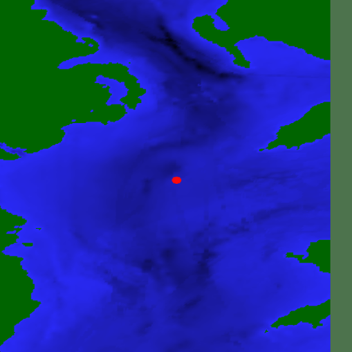
Image 1. A single source in the problem area.
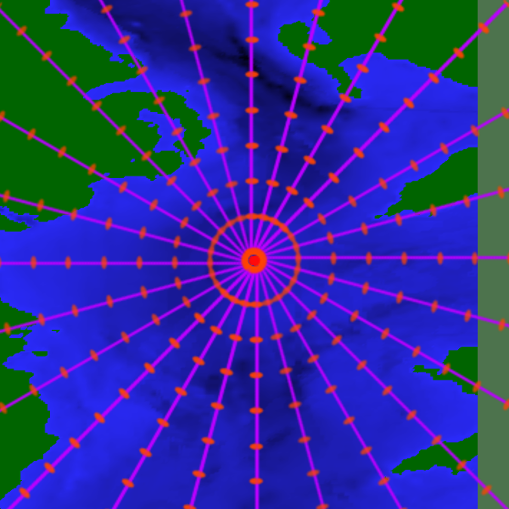
Image 2. Slices and solution points radiating from the source.
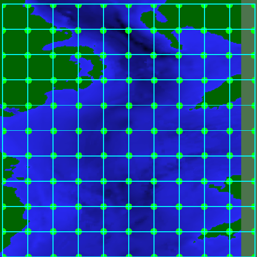
Image 3. The problem grid onto which levels are interpolated.
The overall sound levels are interpolated and summed over all active sources to produce the final grid.