General modelling tips
To navigate, click topic in index to the right or search (Ctrl+f).
This document lays out general tips for modelling underwater noise propagation using for various scenario types. The focus is on enabling the reader to tune their specific model to maintain accuracy while reducing computing cost.
Note that this document is not a guideline for best practice.
1 Definitions
Table 1: Level definitions and the corresponding ISO 18045-2017 reference.
| Unit | Definition | Comments |
|---|---|---|
| SPL (dBRMS) ISO 18405-2017: 3.2.1.1 |
\( \text{SPL} = 10 \cdot \log_{10} \left( \frac{\frac{1}{t_2 - t_1} \cdot \int_{t_1}^{t_2} p(t)^2 \, dt}{1 \cdot 10^{-12} \, \text{𝑃𝑎}} \right) \) | Functionally equivalent to deprecated \( 20 \cdot \log_{10} \left( \frac{\text{RMS}}{1 \cdot 10^{-6} \, \text{Pa}} \right) \) |
| Lp (dBz-p) ISO 18405-2017: 3.2.2.1 |
\( L_p = 20 \cdot \log_{10} \left( \frac{𝑃𝑎_{\text{max}}}{1 \cdot 10^{-6} \, \text{𝑃𝑎}} \right) \) | This assumes that 𝑃𝑎𝑚𝑎𝑥 is equal or greater than \( \sqrt{P_{\text{a min}}}^2 \) |
| Lp-p (dBp-p) | \( L_{p-p} = 20 \cdot \log_{10} \left( \frac{P_{\text{a max}} - P_{\text{a min}}}{1 \cdot 10^{-6} \, \text{Pa}} \right) \) | Often¹ equivalent to 𝐿𝑃 + 6.02 𝑑𝐵 |
| LE (dBSEL) ISO 18405-2017: 3.2.1.5 |
\( \text{LE} = 10 \cdot \log_{10} \left( \frac{\int_{t_1}^{t_2} p(t)^2 \, dt}{1 \cdot 10^{-12} \, \text{𝑃𝑎}} \right) \) | For continuous sound, this is equivalent to \( \text{SPL} + 10 \cdot \log_{10}(t_2 - t_1) \), where \( t \) is in seconds. |
¹ If maximum pulse rarefaction is below ambient pressure and compression and rarefaction phases are of equal size.
- Impulse, signature, time series: A time vs. pressure data series representing an event, typically an impulse.
- Crossover frequency: The frequency at which dBSea switches from its low-frequency solver to its high-frequency solver.
2. Solver Choice and Detail
2.1 Impulsive Noise
If you’re looking to model Lp or Lp-p use dBSeaRay and see sections 3.2, Lp / z-peak, p. 7 & 4.0, Impact Piling, p. 7.
If modelling LE or SPL see section 2.2.
2.2 Non-Impulsive Noise
There is no one-size-fits-all for solver choice but there some general guidelines and some easy checks.
2.2.1 General limits
Table 2: Solver Depth and Frequency Limits
| Solver Name | Depth [m] | Context | Frequency [Hz] | Context |
|---|---|---|---|---|
| dBSeaPE | >50 | dBSeaModes is better at modelling sediment interaction. dBSea might use analytical starter at low depths – not good, change to some other solver. | <1000 | Slow at higher frequencies. |
| dBSeaModes | <1000 | dBSeaModes is very slow in deep or long-range scenarios | <500 | Even slower at higher frequencies. |
| dBSeaRay | >\(\frac{\frac{C_w}{f}}{\left( \frac{\rho_b + C_b}{2000} \cdot 5 - 7 \right)}\) \( C_w \): soundspeed of water. \( \rho_b \): Sediment density. \( C_b \): Water density |
Assumptions for model not met. Calculation produces unrealistic results, neglecting sediment penetration. | Depth-dependent, but generally >250 | Sediment penetration not correctly calculated. |
2.2.2 Check for solver choice and cross-over frequency
Use the probe function to look for discontinuities in received level. We expect received band levels to be 'smooth' if the source band levels are 'smooth'. The correct crossover frequency will lie in the region where the solvers agree on the received level, indicating that both solvers are functioning correctly at that frequency.
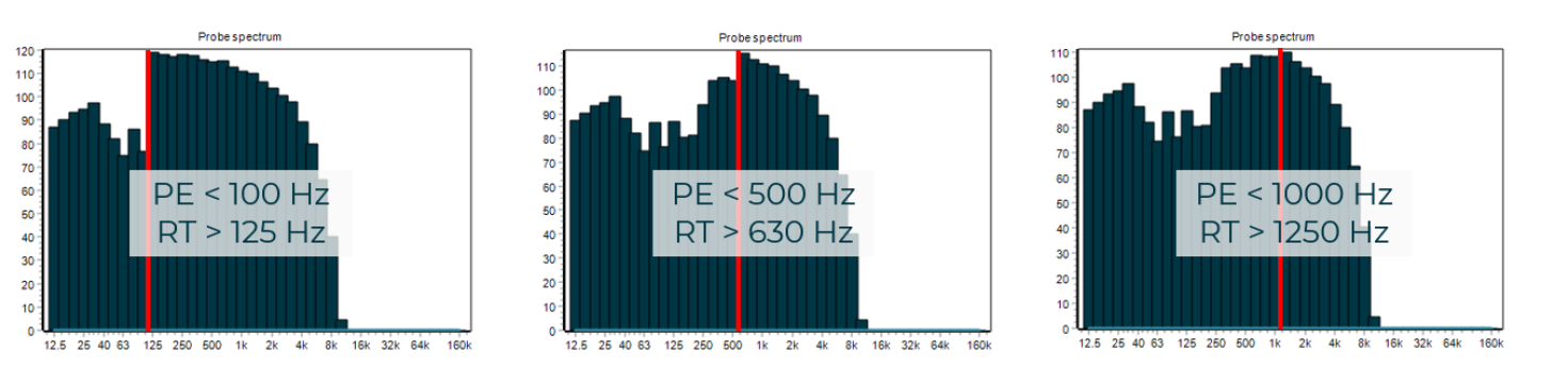
Image 1. Received level at various crossover frequencies for a source where all bands where 200 dB. Solvers 'meet' where crossover frequency is 1000/1250 Hz (right graph), indicating both solvers function correctly there.
2.2.3 Solver resolution/detail
Generally all the solver agree on the propagation loss across a wide range of conditions, if they do not, it’s a sign that you should increase the model resolution either in Setup scenario/Source Solution & z depth points or in Preferences/Advanced.
A notable exception is that we don’t expect dBSeaRay to agree with dBSeaPE or dBSeaModes at low frequencies (~<250 Hz) and high frequencies (~>2000 Hz).
3. Impulsive Noise
3.1 LE / SEL / Exposure Level
3.1.1 Simplest apprach, keep everything in unitless DB
First go to Preferences/Sound levels display and make sure Level type for display is Sound pressure level, dB SPL (Leq).
Yes, do this even if you’re interested in LE results!
The reason we ignore the Sound exposure level option is that it is meant for continuous noise sources where the active duration of the source is important. For the impulsive noise the important metric is the number of impulses.
- When modelling LE from impulses the easiest approach is to do some of the math yourself, as it means you know exactly what to expect from dBSea.
- When importing an impulse signature (time-pressure series) into dBSea, note down the band levels given in the bottom table in the
Time seriesmenu (Image 2, below).
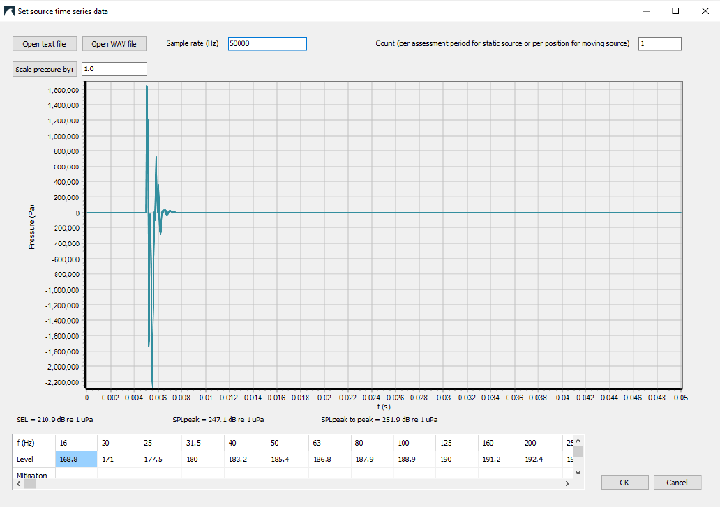
Image 2. Example of an impulse from a 6 m diameter monopile, after import into dBSea.
Paste these band levels into the Spectrum menu Add equipment/New database equipment to get a band-wise representation in dBSea (Image 3). You can now adjust the total level by adjusting the Count (top left cell in Spectrum menu) to the number of impulses in your current event. You do not need to re-solve the scenario after this change. Note that the Spectrum menu might soon be renamed Band levels.
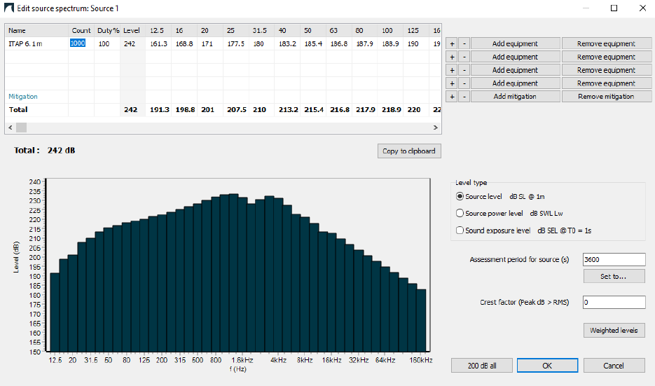
Image 3. Band levels from impulse in Image 2. Note that Total has been adjusted to 1000 blows (count set to 1000, highlighted in blue).
Your results, after solving, will now be the total LE for the number of impulses you have used.
Bonus tip when making impact maps in GIS:
Keep total count to 1 in exports and only export result from 1 impulse. Adjust limits down to reflect more impulses as:
This will speed up the process of generating results for multiple impulse counts as, even though dBSea does not need to re-solve after adjusting count, updating millions of values still take time. It’s much quicker to update a single raster layer colouring in GIS.
3.1.2 Complicated approach, convert to SPL and include time
Get source band levels as described in 3.1.1 above, then convert from LE to SPL by adjusting the LE-single impulse by the impulse repetition frequency (1 divided by time between impulses) as:
E.g. with a repetition every 2 seconds the SPL would be 3.01 dB lower than the LE-single impulse .
In Preferences/Sound levels display set Assessment period for results to the desired time, or set the moving source to the desired time.
3.1.3 Really slow approach
- In
Preferences/Sound levels displaysetLevel type for displaytoSound exposure level. - Set number of impulses in
Count(upper right corner ofTime seriesmenu). - Solve model using dBSeaRay.
3.2 Lp / z-peak
First go to Preferences/Sound levels display and make sure Level type for display is Peak sound pressure level.
3.2.1 Minimal Solve, the Quick Way
-
Go to
Frequencies and solversand setAssessment bandwidthtoOctaveandMaster spectrum FrequenciestoOctave. -
In the
Time seriesmenu, note the band of maximal energy. -
Choose a significance limit, e.g., 16 dB (-0.1 dB in results), and note, starting from the lowest band, where the level reaches the maximal energy minus your limit, e.g.:
- The impulse has the most energy in the band centered on 1000 Hz – LE of 203.6 dB.
- Threshold: 203.6 - 16 = 187.6.
16 dB limit leads to -0.1 dB in overall level:
\[ \text{𝑒𝑟𝑟𝑜𝑟} = 10 \log_{10} \left( 1 - \frac{1}{10^{\frac{16}{10}}} \right) \] -
Going from the band centered on 12.5 Hz, find the first band with a level > 187.6; in this case, that's the band at 63 Hz.
-
Now, from the highest frequency, 8 kHz is the last band > 187.6 dB.
-
Our frequency range is now 63 Hz to 8 kHz. This will be much quicker to model than 12.5 - 160000 Hz, and only -0.1 dB wrong.
We rely on the fact that dBSea propagates the entire impulse regardless, but results are only stored as Lp, with no frequency-specific information.
3.3 SPL / Leq / RMS
Follow steps in section 3.1.2, p. 6, but set total assessment time in Preferences/Sound levels display set Assessment period for results to 1 second (or set moving source to move a total of 1 second).
3.4 SPL instantaneous / SPL 1 sec
Follow steps in section 3.1.2, p. 6.
Before solving go to Preferences/Sound levels display set Sound levels display to Peak sound pressure level.
4. Scenario Types
4.1 Impact Piling
Impact piling can often be done with just 1 mid-water (or mid wet-pile point) source point:
Check that:
- Ranges to relevant receivers are >5x depth at pile.
- Bathymetry is relatively flat.
- You don’t care about the actual sound field close to the source
4.1.1 Fancy moving source piling model
- Use either LE or Lp approach (Impulsive Noise, 3, p. 4) with a moving source with lots of
Sections, moving at the speed of sound of the pile material (e.g. steel, 5000 m/s). - Tick box
Moving sources retain all calculated levels. - Have patience while this solves (!)
- Try to export as animation with
Export/Animated results tool.
4.2 Seismic Surveys
4.2.1 Track modelling
4.2.1.1 Multipoint to One
In a seismic survey individual shot are often very closely spaced, both in time and distance. Also, ranges to impact risks are often much greater than the distance between shots. This means that we can combine several shots into a single multishot, thereby saving modelling time by modelling fewer points in total (see Image 4 below, for concept).
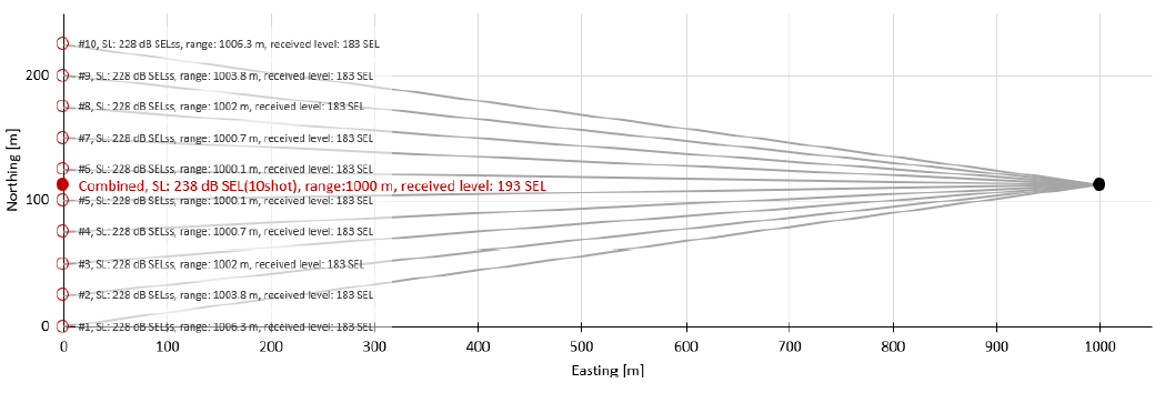 Image 4. 10 source points are
 condensed into one point of source level 10Log10(Npoints) dB higher than the individual points. For receivers far away this is equivalent to having many source points in terms of SEL. Here difference at receiver is <0.02 dB.
Example:
- Shot spacing: 25 m
- Single shot level [LE]: 200 dB
- Number of shots in multishot: 7
- Multishot level [LE]: 208.45 dB
- Receiver range: 500 m
Using the above values we can estimate the difference in doing the calculation per single shot or per multishot:
Table 3. Example of single-shot locations and received levels for a seismic survey.
| Shot Location single-shot X [m] | Shot Location single-shot Y [m] | Range to Receiver [m] | TL (-15 Log10(range)) [LE] | RL [LE] (at location X: 500, Y: 75) Total: 167.9 [LE] |
|---|---|---|---|---|
| 0 | 0 | 505.6 | -40.6 | 159.4 |
| 0 | 25 | 502.5 | -40.5 | 159.5 |
| 0 | 50 | 500.6 | -40.5 | 159.5 |
| 0 | 75 | 500.0 | -40.5 | 159.5 |
| 0 | 100 | 500.6 | -40.5 | 159.5 |
| 0 | 125 | 502.5 | -40.5 | 159.5 |
| 0 | 150 | 505.6 | -40.6 | 159.4 |
Table 4. Example of effect of combining points from above Table 3, to single “multipoint” to simplify modelling.
| Shot Location multishot X [m] | Shot Location multishot Y [m] | Range to Receiver [m] | TL (-15 Log10(range)) [LE] | RL [LE] (at location X: 500, Y: 75) Total: 168.0 [LE] |
|---|---|---|---|---|
| 0 | 75 | 500.0 | -40.5 | 168.0 |
The difference between the two approaches above is <0.1 dB, but the modelling cost has reduced sevenfold. Note that this approach will give you conservative results, as it will increase the shortest impact ranges (where your shot spacing is too large, you’ve combined too many points).
4.2.1.2 Multitrack to One
Just like we can combine several source points into one, we can also combine multiple tracks to a single track (see Image 5). As we get further away from a series of several tracks their combined received level [LE] will approach that of a single track line of a higher source level (equal to the combined energy of the contributing track lines).
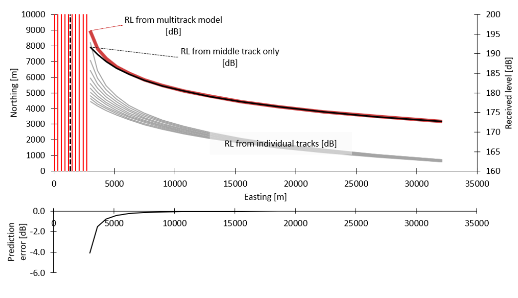
Image 5. A single line with higher source level will have very similar received level to the total received level from all ten tracks, making the modelling of all ten tracks superfluous over medium ranges.
4.2.1.3 Sweep
For seismic surveys we are often interested in the impact range of the broadside emissions from the seismic array, and impact ranges are often measured in multiple kms from the track. This means that calculation of numerous slices/radials that run close to parallel to the track are irrelevant for the impact ranges. For a track that runs from SW to NE at a 45-degree compass heading, setting dBSea to use 8 Radial slices will be enough to ensure that we have modelled the closest point of approach to each point in the scenario. Modelling fewer radials also mean that you can increase the number of shot points in your modelling, while keeping the modelling load reasonable.
Image 6 below shows that with 16 slices/radials we have too many radials simply calculating transmission loss in the direction of travel for the track. We could limit this to 8 radials and get the same result.
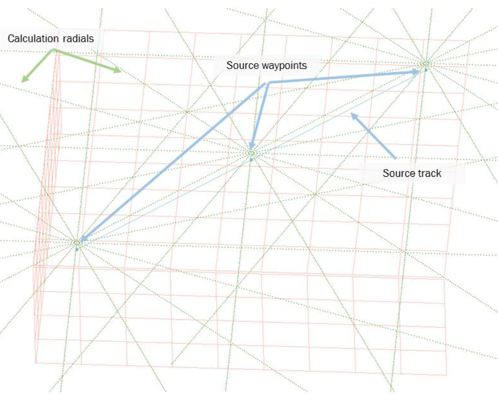
Image 6: Example of a model with 16 slices/radials.